Antonella Basso, Anusha Kumar and Breanna Richards
I. Introduction
Independence is among the most critical assumptions in regression, modeling, and hypothesis testing. In statistics, two events are considered independent iff the occurrence of one has no effect on the probability of the other. Ensuring that sampled data are independent protects us from both making biased population estimates and falling victim to numerous type I errors, or “false positives” (McDonald 2014). That is, false rejections of the null hypothesis when it is in fact true, which in many cases may have dire consequences. To illustrate this phenomenon, consider the following example.
Suppose we are interested in collecting the height measurements of boys and girls in a 4th grade class for comparative estimates of 4th grade students in the US. Our goal is to test whether the mean heights of boys and girls are equal (null hypothesis) against the alternative hypothesis that they are not equal. Suppose further that the null hypothesis is true, and that within the class we’ve chosen to randomly sample, there are three brothers and a pair of identical twin sisters shorter than most of their peers. In conducting the corresponding hypothesis test, we implicitly assume that our data are independent. However, the fact that some of our subjects are biologically related indicates that our data are dependent, as genetics tend to produce similar physical traits (such as height) among kin. This dependence within our data consequently increases our likelihood of wrongfully rejecting the null hypothesis as some of our observations provide additional information about others. That is, our chances of obtaining a p-value less than 0.05 (significance level, \(\alpha\)) is now in fact greater than 5%, making us more prone to committing a type I error.
Scenarios such as this one are rather frequent in the real world and exceedingly difficult to avoid, making the risk of false positives much more prevalent. In this paper we delve further into what happens when the assumption of independence is violated in the context of hypothesis testing. Specifically, we simulate dependent data to explore its effects on false positives and generate plots to illustrate this relationship.
II. Simulation Study
Consider the following data generation process for outcomes \(y_i\), for subject \(i = 1, 2, …, n\):
\[ y_1 \sim N(0,1), \]
\[ y_i \mid y_{i−1} \sim N(\rho \cdot y_{i−1}, 1), \text{for } i=2,…,n. \]
As generated, each observation \(y_i\) and corresponding distribution depends on the former, \(y_{i−1}\) for \(\rho \neq \) 0, giving us dependent sample data. However, note that if \(\rho = 0\), then \(y_1 \sim N(0, 1)\), just as \(y_i \mid y_{i−1} \sim N(0, 1)\) for \(i = 2, …, n\), which not only indicates that the data are independent, but also identically distributed. That is, each observation comes from the same distribution, and thus, has the same expectation, \(\mu\). If, on the other hand, \(\rho\), 0 and the data are dependent, these expectations are no longer constant, meaning that, almost surely, they are not identically distributed. Hence, violating yet another key assumption in hypothesis testing. Together, these assumptions of independence and identical distribution form what is known as independent and identically distributed (or “iid”), which, in practical terms, means that no two observations in any one data set are related and all are taken from the same probability distribution. Now, suppose we observe data \(\{ y_i \}_{i=1:n}\), generated with the DGP outlined above. Our goal is to test the null hypothesis that the mean is zero (\(H_0 : \mu = 0\)), against the alternative hypothesis that the mean is not zero \((H_1 : \mu \neq 0)\). Note that for this study, we hold that the null hypothesis is true.
A. Independent Data
We begin by simulating independent data in R via the DGP mentioned above, setting \(\rho = 0\). Keep in mind that, as mentioned, this means that our data is (\(y_i \sim N(0, 1)\), for \(i = 1, …, n\)) and hence, the expected value of \(y\) remains zero, namely \(\text{E}[Y] = \mu = 0\). Specifically, we generate 1,000 data sets of sample size \(n = 1,000\), and for each, we run a t-test with unknown variance, recording the decision to accept or reject the null hypothesis based on a type I error rate of \(\alpha = 0.05\). That is, for each data set, we generate a corresponding p-value and compute the proportion, which we denote \(\hat{\alpha}\)), of those which exceed our significance level of 0.05 out of the total 1,000 decisions made. As expected, doing so yielded \(\hat{\alpha} = 0.048 ≈ 0.05\), indicating that nearly 5% of the 1,000 t-tests conducted incorrectly rejected the null hypothesis, assumming that \(H_0\) is true. And, given that our data are iid, obtaining a type I error rate close to 0.05 demonstrates that the t-test assumptions are met, thus producing t-statistics that follow a t-distribution (more on this later).
B. Dependent Data
Seeing how independent data yields results that conform to the t-test assumptions, we now proceed by increasing the value of \(\rho\) to observe the influence of dependent data on \(\hat{\alpha}\). As before, we simulate 1,000 data sets with \(n = 1,000\), this time with \(\rho \in \{0, 0.1, 0.2, …, 0.9\}\), resulting in a total of ten simulations, and hence, ten \(\hat{\alpha}\) values, one for each value of \(\rho\). The graph below illustrates the change in \(\hat{\alpha}\) for each incremental change in \(\rho\).
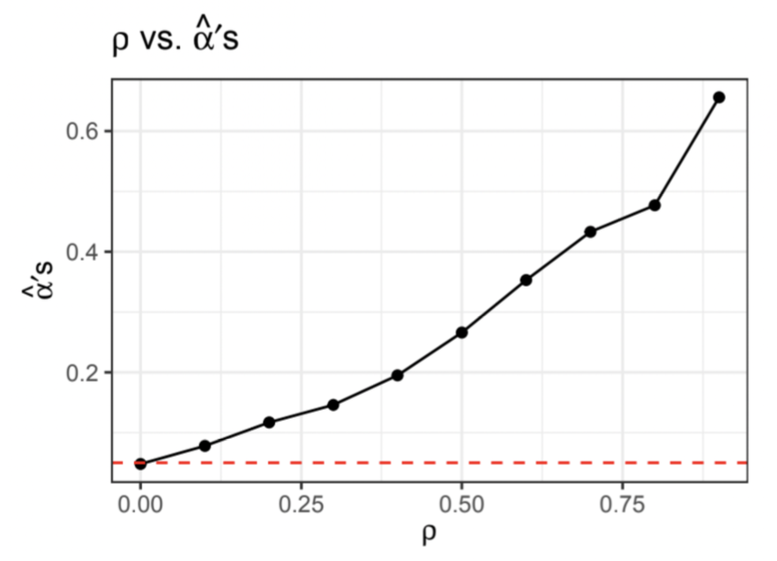
Notice that the proportion of times we incorrectly reject the null hypothesis increases, almost exponentially, as we increase the value of \(\rho\). In fact, the type I error rate is only at most 0.05 when \(\rho = 0\). Given that our \(\alpha\)-level is set at 0.05, we expect there to be approximately a 5% likelihood of rejecting the null hypothesis by chance. However, this graph shows us that we are in fact far more likely to make type I errors when our data are dependent. Thus, in an official study, we would be wrong in asserting that we’ve not made this kind of error 95% of the time.
C. Comparing Distributions
As mentioned previously, independent data produce t-statistics that assume a t-distribution. Yet, dependent data violate this assumption in yielding type I error rates that are, in reality, much greater than we’d expect. To illustrate this, we simulate 1,000 data sets with \(n = 1,000\) as before, but with \(\rho = 0, 0.5, 0.9\). Again, we run 1,000 t-tests for each simulation and value of \(\rho\), but rather than recording their p-values with which to compute a proportion of null rejections, we instead obtain their corresponding t-statistics so as to plot them against a theoretical t-distribution. It is important to note that a t-statistic is a measure of how extreme a statistical estimate, such as the mean, is when compared to a hypothesized population parameter, such as the null hypothesis (Simon 2000). Thus, in our case, t-statistics close to zero indicate their proximity to the true mean. The graphs below show the frequency distributions of these t-statistics for each of the three values of \(\rho\) against the theoretical t-distribution (in red) with \(n − 1 = 999\) degrees of freedom.
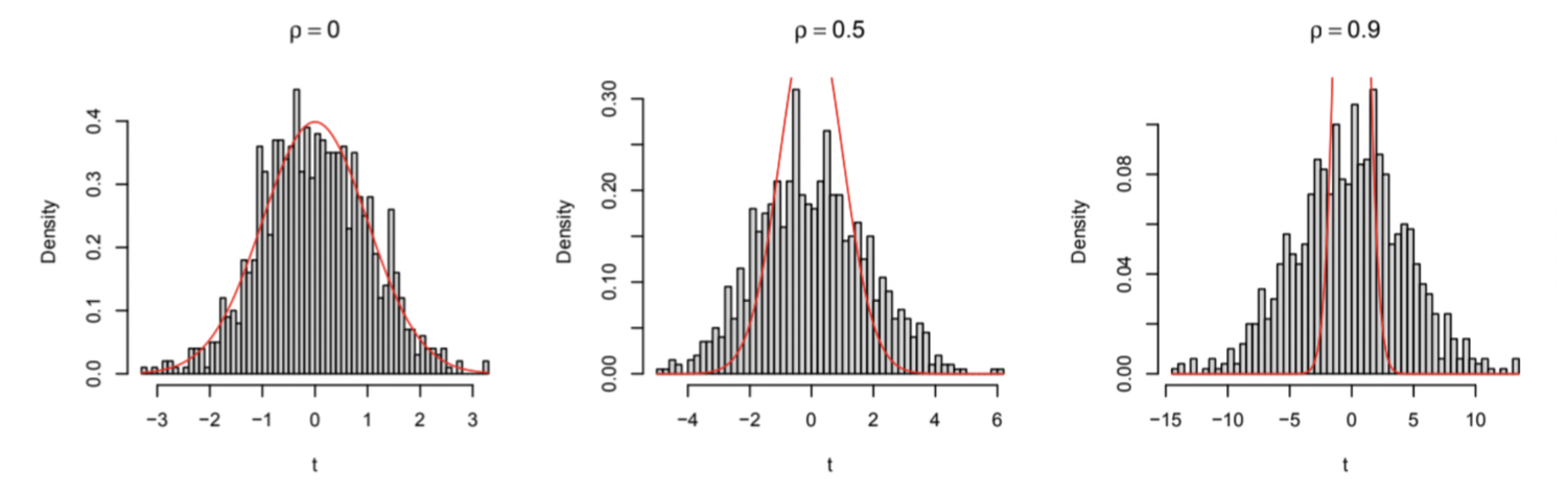
Given that t-statistics of larger magnitudes are less likely to be observed, the left and right tails of the t-distribution correspond to instances of obtaining more extreme values of \(t\). Hence, assuming that the null hypothesis is true, the probability of observing more extreme t-statistics should be very small in accordance with the theoretical t-distribution. Here however, we see that as we increase \(\rho\), we observe higher volumes of extreme t-statistics. In turn, we become less likely to observe statistics close to our hypothesized population parameter, \(\mu = 0\). Moreover, notice that when \(\rho = 0\), the distribution of t-statistics fits the theoretical t-distribution, which further validates our previous observation that only about 5% of the data was rejected under the null hypothesis. However, we see that when we increase \(\rho\), the distribution of t-statistics begins to expand beyond the theoretical t-distribution. This coincides with the increase in \(\hat{\alpha}\) values, or incorrect null rejections, we observed previously, as more and more t-statistics extend towards our rejection region and the share of falsely rejected nulls becomes larger. Specifically, the previous graph showed that the proportion of falsely rejected nulls was roughly 70% when we set \(\rho = 0.9\). Similarly, in the right-most histogram above, we see that approximately the same share of t-statistics lie within the rejection region and outside the t-distribution assumed under the t-test. This further supports the notion that as our observations become more dependent, the rate at which we falsely reject the null hypothesis increases.
III. Conclusion
T-tests are among the many statistical tests that rely on the assumption of iid data. As we have shown, when observations in our samples provide additional information about others, this assumption is violated in that they are no longer mutually independent. This implicit dependency, further suggests that our samples are not drawn from the same probability distribution. Therefore, hypothesis testing with dependent data increases our type I error rate when the null hypothesis is true. Nonetheless, the iid assumption is rather unrealistic in practical statistical applications as repeated measures and related samples are quite common in the real world. For example, a study may be interested in taking the blood pressure readings of a group of individuals before and after a drug dosage. We expect these pairs of observations to be correlated because they come from the same individual, meaning that the data are not mutually independent (See How are dependent and independent samples different?). Another example would be a study tracking the outcomes of infectious disease status. One person’s disease status is likely to affect another’s if they maintain close contact like living in the same household or sharing the same workplace. In this case, the iid assumption is violated if there are repeated measurements or if there is contact between individuals. And, as we’ve demonstrated, not only does the violation of this crucial assumption cause us to make false positive conclusions far more frequently, but it drives us to make inaccurate claims about the rate at which we make them, something that could prove to be far more disastrous depending on the situation. In public health and medical research, this elevated risk of type I errors may lead to a rise in the acceptance of unnecessary policies or interventions, wasting valuable time and resources (Mcleod 2019). For instance, they could “cause the appearance that a treatment for a disease has the effect of reducing the severity of the disease when, in fact, it does not”, bringing about a chain of wasteful and life-altering repercussions (Kenton 2022). For this reason, careful data collection is vital to upholding statistical accuracy and integrity in scientific research. Although we may not be able to change the condition of our data, understanding its implications before engaging in scientific study could save us from making false assumptions that could negatively impact the lives of others.
References
- McDonald, J.H. (2014). Independence. Handbook of Biological Statistics (3rd Edition), pp. 131-132. Sparky House Publishing, Baltimore, Maryland. ISBN-13 978-1-478-63789-9.
- Simon, S. (2000, September 18). StATS: What is a t statistic? P.Mean. http://www.pmean.com/definitions/tstat.htm
- How are dependent and independent samples different? (n.d.). Minitab 21 Support. https://support.minitab.com/en-us/minitab/21/help-and-how-to/statistics/basic-statistics/supporting-topics/tests-of-means/how-are-dependent-and-independent-samples-different/
- Mcleod, S. (2019, July 4). What Are Type I and Type II Errors? Simply Psychology. https://www.simplypsychology.org/type_i_and_type_ii_errors.html
- Kenton, W. (2022, November 27). Type 1 Error: Definition, False Positives, and Examples. Investopedia. https://www.investopedia.com/terms/t/type_1_error.asp
Code Appendix
## Libraries
library(tidyverse)
library(latex2exp)
## II.A Independent Data

set.seed(1)

## Data Generating Process
dgp <- function(rho){
#' data gen. process (dgp) function generates a dataset of size 1,000 for given rho
#'@param rho sets value of rho
#'@return test TRUE/FALSE indicating when a rejection of the null is made

  # pull y_1 from N(0,1)
  y <- c(rnorm(1, 0, 1))

  # pull y_i from N(rho*y_{i-1}, 1) for i > 2
  for (i in 2:1000){
    y[i] <- rnorm(1, rho*y[i-1], 1)
    }

  # run t-test and return TRUE if p-value <= 0.05
  test <- ifelse(t.test(y)$p.value <= 0.05, TRUE, FALSE)
  return(test)
}

# find proportion of times we reject the null hypothesis (alpha hat)
alpha_hat <- sum(replicate(1000, dgp(0), simplify=T))/1000
## II.B Dependent Data

set.seed(1)

# test rho values from 0 to 0.9 in increments of 0.1
rho_seq <- seq(0, 0.9, 0.1)

# find proportion of null rejections for each rho in rho_seq (alpha hats)
alpha_hats <- c()
for (i in 1:length(rho_seq)){
  alpha_hats[i] <- sum(replicate(1000,
                                 dgp(rho_seq[i]),
                                 simplify=T))/1000
 }
## Plot 1

# save data frame of rho's vs. alpha hats
plot_b <- as.data.frame(cbind(rho_seq, alpha_hats))

# plot rho's vs. alpha hats
ggplot(plot_b, aes(x=rho_seq, y=alpha_hats)) +
  geom_point() + geom_line() +
  geom_hline(yintercept=0.05, linetype="dashed",
             color="red", size=0.5) +
  labs(title=TeX('$\\rho$ vs. $\\hat{\\alpha}\'$s'),
       x=TeX('$\\rho$'),
       y=TeX('$\\hat{\\alpha}\'$s')) + theme_bw()
## II.C Comparing Distributions

set.seed(1)

## Data Generating Process 2
dgp_t <- function(rho) {
#' dgp_t function generates dataset of size 1,000 for a given rho and
#' returns t-statistic from two-sided t-test
#'@param rho sets value of rho
#'@return t-statistic value

  # pull y_1 from N(0,1)
  y <- c(rnorm(1, 0, 1))

  # pull y_i from N(rho*y_{i-1}, 1) for i > 2
  for (i in 2:1000){
    y[i] <- rnorm(1, rho*y[i-1], 1)
    }

  test <- t.test(y)$statistic
  return(test)
}

# rho values to collect t-statistics for
rho_seq2 <- c(0, 0.5, 0.9)

# collect 1,000 t-statistics for each rho in rho_seq2
t_stats <- replicate(1000, sapply(rho_seq2, dgp_t), simplify=F)

# arrange t-statistics into a matrix
t_stats <- matrix(unlist(t_stats), ncol=3, nrow=1000, byrow=T)
## Plot 2

# plot side-by-side histograms of t-statistics for rho={0, 0.5, 0.9} and overlay t-distribution with 999 degrees of freedom
par(mfrow=c(1,3))

# rho=0
hist(unlist(t_stats[,1]),
     freq=FALSE, breaks=50,
     xlab="t", main=TeX('$\\rho = 0$'))
curve(dt(x, df=999), add=TRUE, col="red")

# rho=0.5
hist(unlist(t_stats[,2]),
     freq=FALSE, breaks=50,
     xlab="t", main=TeX('$\\rho = 0.5$'))
curve(dt(x, df=999), add=TRUE, col="red")

# rho=0.9
hist(unlist(t_stats[,3]),
     freq=FALSE, breaks=50,
     xlab="t", main=TeX('$\\rho = 0.9$'))
curve(dt(x, df=999), add=TRUE, col="red")