I. Introduction
Despite explicit laws to protect against lending discrimination—such as the Fair Housing Act (FHA), the Equal Credit Opportunity Act (ECOA),
and the Community Reinvestment Act (CRA) (Folger 2022)—Black families in the US continue to face alarming levels of injustice in loan lending scenarios, which exacerbates racial inequities like those of homeownership. Specifically, when lenders choose to ignore an individual’s race in making decisions, instead using income and credit score as a basis for loan approval, they ignore the prominent role that systemic racism plays in economic disparity and implicitly contribute to widening the racial wealth gap (Reynolds, Perry and Choi 2021). In an attempt to bring attention to our nation’s racially disproportionate and systemic denial of loans that harms American citizens and prevents wealth building in communities of color, this analysis aims to utilize hierarchical Bayesian modeling to gauge the degree of discrimination in loan lending decisions across all 50 states. In addition to discussing the data used for estimating our parameters of interest, we outline our chosen model as well as its implementation using an MCMC algorithm, and discuss our results. Ultimately, we hope to show how Bayesian methods may be used to infer about our institutional decision making practices and not only discover discrimination but estimate it in a way that may influence more adequate and substantive policies.
II. Data
The data used for this analysis, obtained from the Consumer Financial Protection Bureau, spans thousands of 2017 loan application records from
financial institutions across the US that have been made publicly available under the Home Mortgage Disclosure Act (HMDA) (Download HMDA Data). The records gathered reflect individual applications wherein one of the following eight potential actions were taken (A Guide To HMDA Reporting: Getting It Right!).
- Loan originated
- Application approved but not accepted
- Application denied by financial institution
- Application withdrawn by applicant
- File closed for incompleteness
- Loan purchased by the institution
- Preapproval request denied by financial institution
- Preapproval request approved but not accepted (optional reporting)
Given our focus on individuals whose applications were either approved or denied, we filter out observations involving actions 1, 4, 5, or 8,
and categorize those pertaining to actions 2 or 6 and actions 3 or 7 as approved and denied cases, respectively. Moreover, as we are interested
in lending differences between Black and white applicants specifically, we also exclude individuals from other racial groups as well as those
who did not specify group membership from our analysis. Having compiled and preprocessed the data to reflect the proportions of Black and white
applicants that were approved for a loan, we are left with two observations for each of the 50 states—one for each racial group—totaling
100 observations for the 2017 year.
III. Model
Under a causally-motivated understanding of discrimination, we seek to estimate the effect of racial group membership (Loftus et al. 2018) on one’s chances of being approved for a loan within a given state. Specifically, we wish to determine whether loan approval rates vary systematically as a function of racial group membership across states. Thus, given these aims and the nature of our data, we implement a hierarchical binomial model for clustered data similar to that adopted by Jackman (2009) in an analysis of a cluster-randomized experiment (Green and Vavreck 2008) for “assessing the effects of a voter mobilization treatment in the 2004 US presidential election” (Jackman 2009). For our purposes, we assume observations are clustered by state and that each cluster comprises two observations, namely, 2017 count data for each racial group of interest.
Focusing on the success rate to guide our estimation of discriminatory effects in loan approval across states, we implement the following hierarchical binomial model. For \(i = 1,2,…,100\), let \(n_i\) be the total number of applicants and \(r_i\) be the number of approvals such that \(p_i = r_i / n_i\) gives the \(i\)th observation’s approval rate. Moreover, let \(S_i \in \{1,2,…,50\}\) be the state indicator and \(W_i \in \{0, 1\}\) be the racial group indicator for observation \(i\), such that \(S_i = 1\) and \(W_i = 1\) jointly denote the white racial group observation for the first state alphabetically—Alabama (AL). Assuming normally distributed effects \(\alpha_{S_i}\) and \(\delta_{S_i}\) with normal mean parameter densities \(\mu_{\alpha}\) and \(\mu_{\delta}\), we have
\[ r_i \sim \text{Bin}(n_i,p_i), \]
\[ \text{logit}(p_i) = \alpha_{S_i} + \delta_{S_i}W_i, \]
\[ \alpha_{S_i} \sim \text{N}(\mu_{\alpha},\sigma_{\alpha}^2), \]
\[ \delta_{S_i} \sim \text{N}(\mu_{\delta},\sigma_{\delta}^2), \]
\[ \mu_{\alpha} \sim \text{N}(0,2^2), \]
\[ \mu_{\delta} \sim \text{N}(0,2^2), \]
\[ \sigma_{\alpha} \sim \text{Unif}(0,2), \]
\[ \sigma_{\delta} \sim \text{Unif}(0,2), \]
where \(\sigma_{\alpha}^2\) and \(\sigma_{\delta}^2\) are the hierarchical variance parameters. We assume noninformative uniform hyperpriors on \(\sigma_{\alpha}\) and \(\sigma_{\delta}\), which according to Gelman et al. (2014) should not result in an improper posterior density due to the large number of clusters in the data, and posed no problems for Jackman (2009) despite nonconjugacy.
Given our lack of information to distinguish between the \(n_i\) applicants for each observation, we take lending decisions to be exchangeable Bernoulli trials, each given a success rate of \(p_i\), and like Jackman (2009), implement a binomial model for loan approvals \(r_i\) at the observation level, assuming these are independent conditional on \(p_i\). Additionally, aside from state name and racial group, the fact that we lack information to differentiate between state observations allows us to both assumme exchangeability for \(p_i\) conditional on \(S_i\) and \(W_i\), as well as model state-level effects exchangeably with a common prior distribution as shown above.
As we are unsure about the degree of discrimination present on both state and national levels purely from the records collected for the 2017 year—themselves subject to preprocessing error—we remain ambiguous about discriminatory effects so as to allow the data to play a larger role in informing us about state-level variations in racial discrepancies of loan approval rates. For this reason, we assign normal priors to the baseline levels \(\alpha_{S_i}\) and discriminatory effects \(\delta_{S_i}\), supposing that their expected values are also normally distributed with mean 0. Specifically, since the assumption that \(\text{E}[\delta_{S_i}] = 0\) is rather optimistic regarding discrimination, we instead posit that the ground truth must be a compromise between the observed data, our knowledge of existing systemic racism, and what we ought to expect given the aforementioned policy interventions. As such, we hold that our assumptions that \(\text{E}[\delta_{S_i}] = \mu_{\delta}\) and \(\text{E}[\mu_{\delta}] = 0\), with given variances, better capture our uncertainty about the extent of discrimination in these contexts.
IV. Implementation
Similar to the methodology proposed by Jackman (2009), we implement our hierarchical model within a single-chain MCMC algorithm to generate posterior estimates of the state-level effects and corresponding hyperparameters. Using the rjags package for our implementation, we give all parameters initial values of 0 and generate 50,000 samples after a 1,000 iteration burn-in, subsequently saving every fifth iteration for inference.
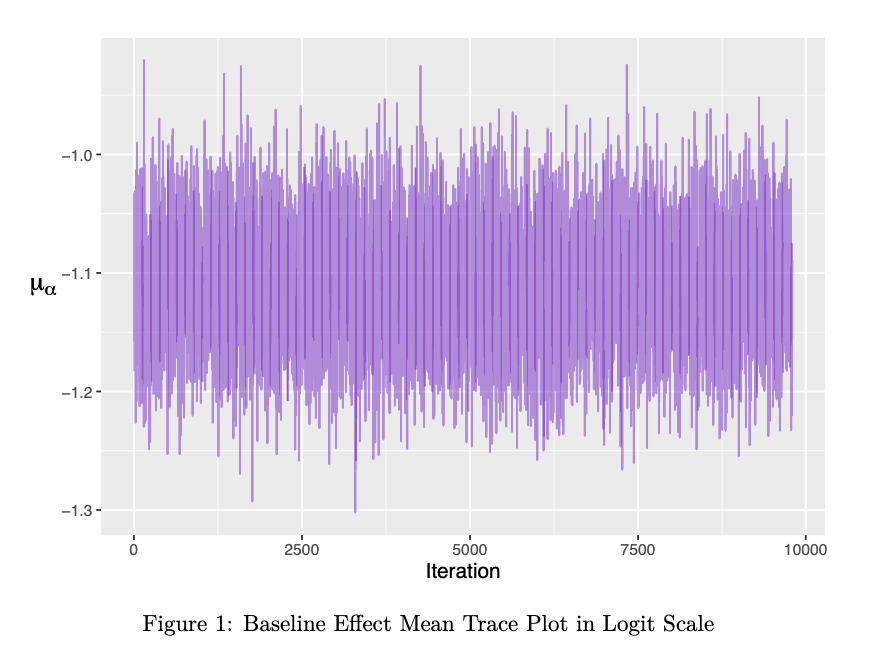
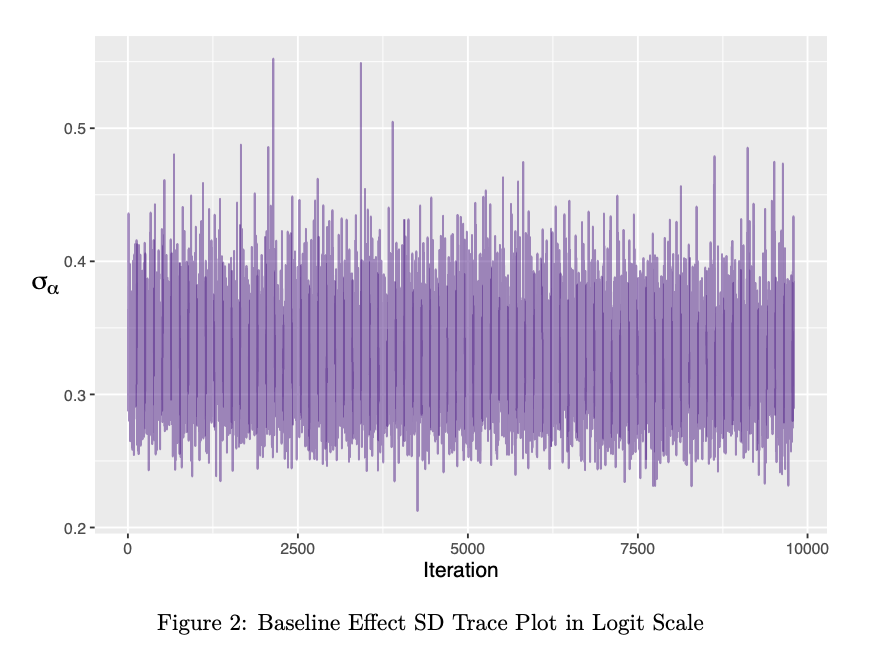
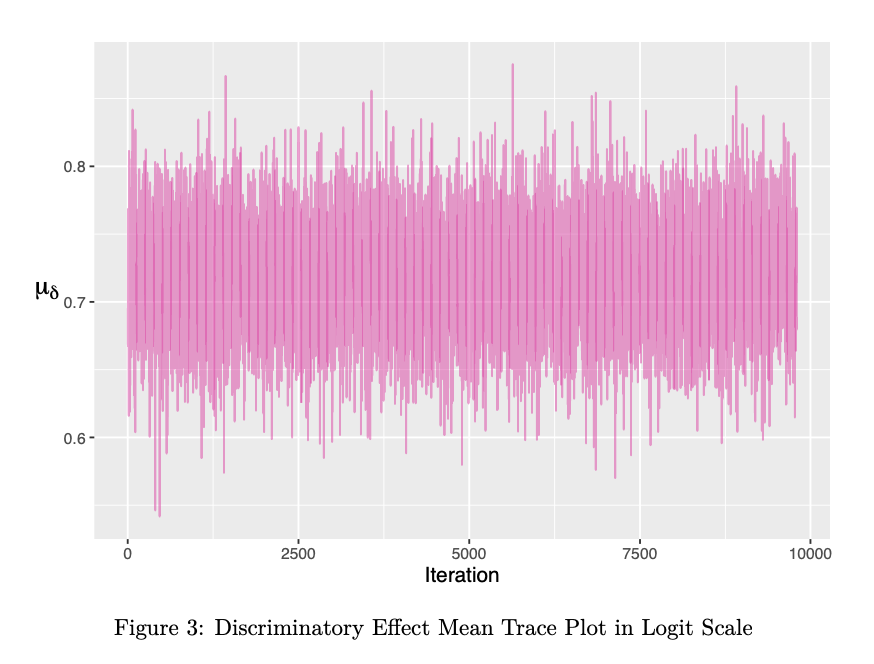
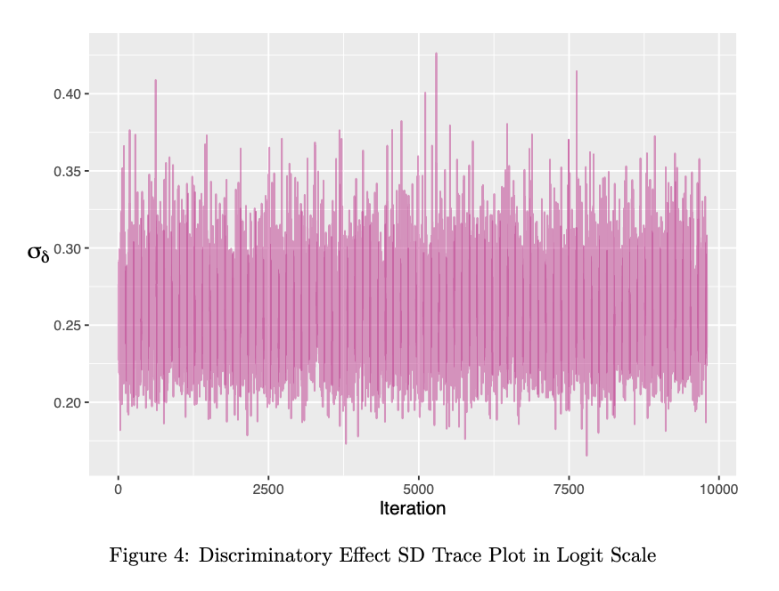
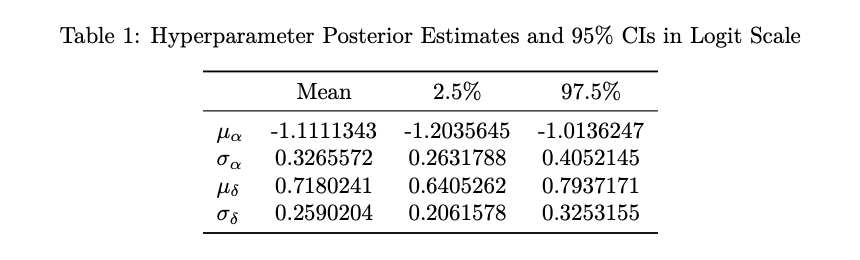
Figures 1-4 demonstrate that our chain successfully converges to the target posterior densities rather quickly, seeing as parameter values remain stabilized after burn-in. Given the large number of effect parameters in our model, we only provide trace plots for the hyperparameters as they reflect similar states of achieved convergence. Table 1 provides their corresponding posterior estimates as means of the 10,000 saved samples and 95% highest density region (HDR) credible intervals. Notably, we see little posterior uncertainty in \(\sigma_{\delta}\) despite the much larger 95% HDR interval for \(\mu_{\delta}\). However, with a posterior mean of approximately 0.72 and a credible interval that still does not contain 0, it follows that our model supports the intuition that positive state-level discriminatory effects in fact exist across states on average.
For comparison, we generate maximum likelihood estimates (MLE) of the state-level effects via a standard generalized linear model with a logit link function. The forest plot given by Figure 5 below displays these point estimates along with their 95% confidence intervals for each state in order from highest to lowest effect estimate. As shown, we include our posterior estimates from the hierarchical binomial (HB) model and corresponding 95% HDR intervals to see the extent to which our assumed hierarchical model and prior beliefs about the parameters align with the observed data.

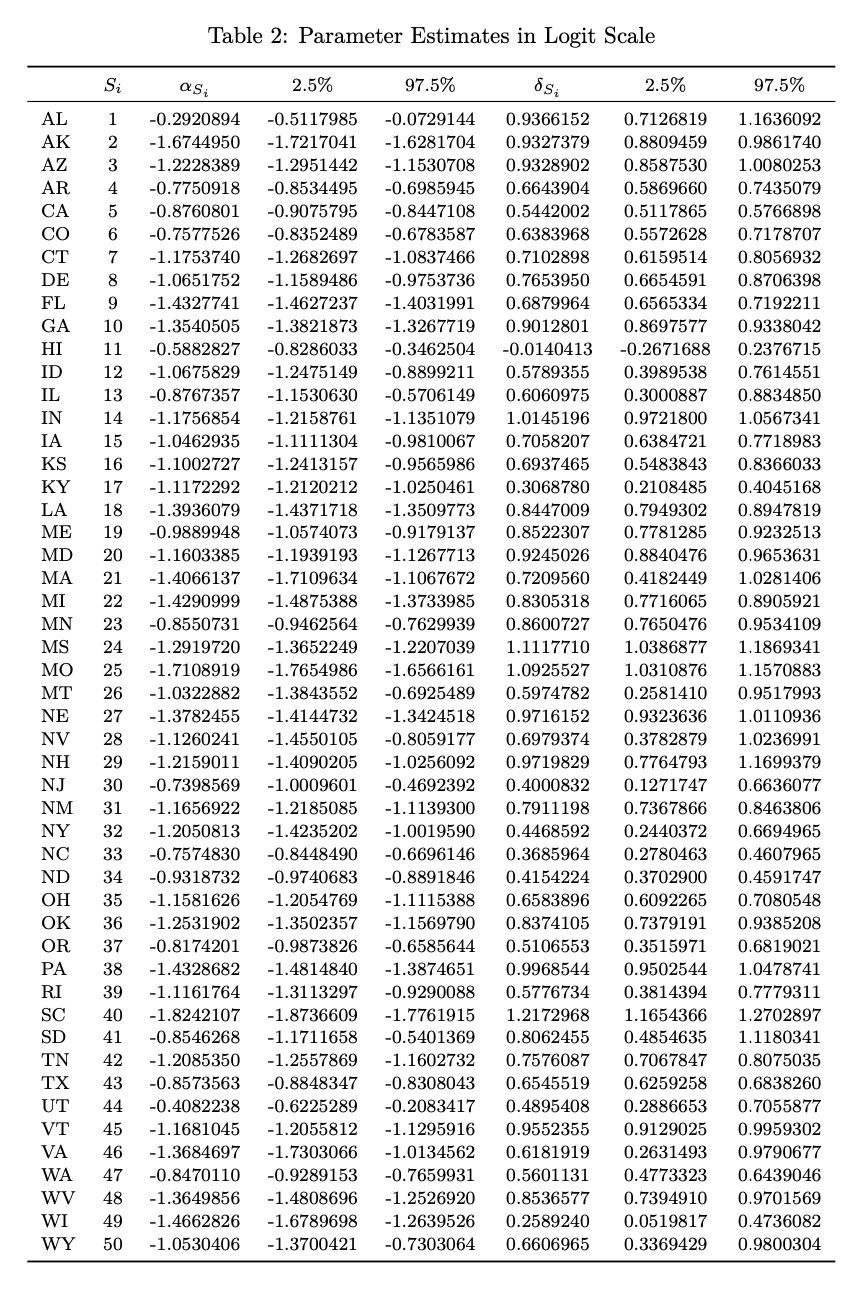
Alarmingly, but not surprisingly, all states with the exception of Hawaii (HI) demonstrate positive average discriminatory effects for both estimators. While our posterior estimates are rather similar to those obtained via standard MLE, especially for large values of \(\delta\), we see that the HB estimates are generally larger with means slightly above those of MLE and display less variability overall with more shrinkage towards the average effect. Notably, this suggests that there isn’t significant posterior uncertainty in our parameters despite our use of relatively diffuse priors. Table 2 below gives our MCMC-generated effect estimates for all 50 states along with their respective 95% HDR intervals.
V. Evaluation
Given our specific focus on the discriminatory effects, we further assess the fit of our model by using the posterior distribution to generate out-of-sample discriminatory effect predictions for an average state and a new hypothetical state with corresponding p-values. We find that the average state has a posterior probability close to 1 for having a discriminatory effect greater than 0. While this further validates the presence of discrimination in US loan lending decisions and suggests that the observed data is very likely under our posterior distribution, it is possible for the extremity of the p-value to be indicative of overfitting, especially given our restriction to a single year and complex hierarchical structure.
Simulating a new discriminatory effect \(\delta_{\text{new}}\) for a hypothetical state, we see that although it is approximately equal to the posterior mean of \(\mu_{\delta}\approx 0.72\) on average, it has a much narrower 95% HDR interval, as shown in Table 3 below. Moreover, while this new effect also yields a posterior predictive p-value close to 1, it is in fact smaller for the average state-level effect, therefore providing more hope for predictive potential. It should be noted however that such a result still does not rule out the possibility of overfitting entirely.
\[\text{P}(\delta_{\text{new}} \ge 0) \approx 0.9967\]
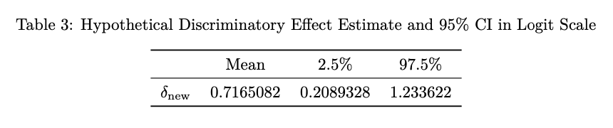
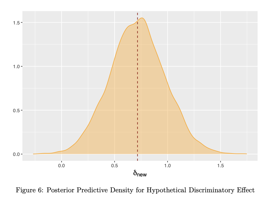
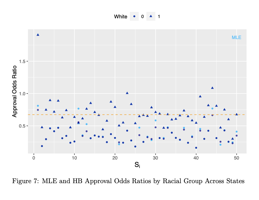
Figure 6 gives the posterior predictive density for \(\delta_{\text{new}}\) generated from 10,000 sampled predictions. Additionally, Figure 7 gives the posterior odds ratios of loan approval for each racial group across states along with those observed in the data. Overall, it is evident that states reflect not only significant, but pretty consistent levels of discrimination, further justifying our choice to model effects exchangeably.
VI. Discussion
Through hierarchical Bayesian modeling, we estimated the degree of discrimination in loan lending decisions in the US, which more than showing the benefits of these methods in making inferences about the systematic and underacknowledged oppression of marginalized groups, provides meaningful insights into the variation of discriminatory practices across the country. Specifically, our analysis reveals strong evidence of discriminatory lending decisions against Black applicants, with estimated odds ratios of approval ranging from 0.16 to 1.91 across states—findings which highlight the presence of continued racial disparity in access to credit and its detrimental impact on Black individuals and communities.
Aside from potential overfitting, our model and subsequent analysis is subject to other limitations worth considering. First, the data used only pertains to applicants in the 2017. It is possible, although not likely, for patterns in application and lending decisions to have since changed. It would thus we worth fitting a similar model to data that is reflective of more recent years or longer periods of time. Second, our analysis only focused on Black and white applicants for the purpose of addressing the perpetual neglect of a historically targeted group in this country. However, we acknowledge that future studies should explore discrimination against other minority groups. Additionally, our data reflect a considerable imbalance in racial groups across states with white applicants constituting the majority of observations. This however does not suggest that there more white individuals applied for loans, but rather that more white compared to Black applicants actually chose to disclose their racial group membership. And, although this doesn’t necessarily influence the approval rates observed \(p_i\), it could have introduced some bias into our estimates.
Due to the fact that we exclude income and creditworthiness from our model, the estimated and discussed discriminating effect(s) reflect both direct and indirect forms of racism that are partially related to systemic bias and ongoing income inequality in this country. Thus, to estimate the (direct) effect of disclosed racial group membership on one’s chances of being approved for a loan—that is, unmediated by economic status—one would have to include and adjust for additional financial predictors \(X\) in the model. To this end, it would make sense to model \(r_i\) conditional on \(x_i\) as well as \(p_i\), since \(r_i|x_i,p_i\) maintains exchangeability among \((r_i,x_i,p_i)\) and allows us to assume a common prior distribution (Gelman et al. 2014). Another potential extension to this work may be to change our prior distrubutions to reflect our knowledge about state-level characteristics, such as predominant political affiliation, or to assume more informative priors that better account for existing patterns of lending discrimination as well as the role of systemic racism in such practices.
Despite the limitations discussed, our results suggest that lending discrimination is a persistent problem with detrimental consequences for the affected individuals and communities. Furthermore, our model provides a framework for quantifying and understanding the potential impact of systemic racism on lending decisions. By highlighting its role in the lending industry and all of its downstream effects, we hope to influence more equitable and informed policy decisions to address this issue and create a more equitable lending environment for all Americans.
References
- Folger, J. (2022, August 14). The History of Lending Discrimination. Investopedia. https://www.investopedia.com/the-history-of-lending-discrimination-5076948
- Reynolds, L., Perry, V. and Choi, J.H. (2021, October 13). Closing the Homeownership Gap Will Require Rooting Systemic Racism Out of Mortgage Underwriting. Urban Institute. https://www.urban.org/urban-wire/closing-homeownership-gap-will-require-rooting-systemic-racism-out-mortgage-underwriting
- Download HMDA Data. (n.d.). Consumer Financial Protection Bureau. https://www.consumerfinance.gov/data-research/hmda/historic-data/?geo=wy&records=all-records&field_descriptions=codes
- A Guide To HMDA Reporting: Getting It Right! (2023, January 1). Federal Financial Institutions Examination Council. https://www.ffiec.gov/hmda/guide.htm
- Loftus, J.R., Russell, C., Kusner, M.J. and Silva, R. (2018, May 15). Causal Reasoning for Algorithmic Fairness. https://doi.org/10.48550/arXiv.1805.05859
- Green, D.P. and Vavreck, L. (2008). Analysis of Cluster-Randomized Experiments: A Comparison of Alternative Estimation Approaches. Political Analysis (Volume 16, 2nd Edition) pp. 138–152. Cambridge University Press. https://doi.org/10.1093/pan/mpm025
- Jackman, S. (2009). Hierarchical Statistical Models. Bayesian Analysis for the Social Sciences, pp. 299–378. John Wiley & Sons, Ltd. ISBN 978-0-470-68662-1.
- Gelman, A., Carlin, J.B., Stern, H.S., Dunson, D.B., Vehtari, A. and Rubin, D.B. (2014). Hierarchical Models. Bayesian Data Analysis (3rd Edition), pp. 101–132. Chapman and Hall/CRC. ISBN-13 978-1-439-84095-5.
Code Appendix
## Libraries
library(tidyverse)
library(latex2exp)
library(kableExtra)
library(tidybayes)
library(R2jags)
library(lattice)
## Compiling Data

get_nums <- function(state){
#' function obtains the desired data and parameters of interest for a given state (2 total observations, 1 for each racial group)
#'@param state is a number between 1-50 referencing a given state's abbreviation when ordered alphabetically
#'@return list(b=b, w=w) is a list of 2 vectors corresponding to the racial groups of interest (b/w = 0/1)

  data <- read.csv(paste0("~/HMDA/hmda_2017_", state.abb[state], ".csv")) %>%
    select("action_taken", "applicant_race_1")

  data <- data[data$action_taken %in% c(2, 3, 6, 7) & data$applicant_race_1 %in% c(3, 5),]

  r_b <- nrow(data[data$applicant_race_1==3 & data$action_taken %in% c(2, 6),]) # total black approved
  n_b <- nrow(data[data$applicant_race_1==3,]) # total black
  p_b <- r_b/n_b # prop. black approved

  r_w <- nrow(data[data$applicant_race_1==5 & data$action_taken %in% c(2, 6),]) # total white approved
  n_w <- nrow(data[data$applicant_race_1==5,]) # total white
  p_w <- r_w/n_w # prop. white approved

  b <- c(0, r_b, n_b, p_b)
  w <- c(1, r_w, n_w, p_w)

  return(list(b=b, w=w))
}

loans_b <- data.frame(state=state.abb,
                      white=rep(0, 50),
                      r=rep(0, 50),
                      n=rep(0, 50),
                      p=rep(0, 50))

loans_w <- data.frame(state=state.abb,
                      white=rep(1, 50),
                      r=rep(0, 50),
                      n=rep(0, 50),
                      p=rep(0, 50))

for (i in 1:50){
  for (j in 1:4){
    loans_b[i, j+1] <- get_nums(i)$b[j]
    loans_w[i, j+1] <- get_nums(i)$w[j]
    }
  }

# merging data
loans <- rbind(loans_b, loans_w) %>% arrange(state, white)

stateIndex <- c(1)
for (i in 2:100){
  if (loans$white[i]==1){
    stateIndex <- c(stateIndex, tail(stateIndex, 1))
    } else {
      stateIndex <- c(stateIndex, tail(stateIndex, 1)+1)
    }
  }

whiteIndex <- c(1, 1)
for (i in 3:100){
  if (loans$white[i]==0){
    whiteIndex <- c(whiteIndex, tail(whiteIndex, 1))
    } else {
      whiteIndex <- c(whiteIndex, tail(whiteIndex, 1)+1)
    }
  }

loans <- loans %>% mutate(whiteIndex=whiteIndex, stateIndex=stateIndex)
## Hierarchical Binomial Model (JAGS)

# Defining Model
sink("model_loans.txt")
cat("
model {

  for (i in 1:100){
    logit(p[i]) <- v[i]
    v[i] <- alpha[stateIndex[i]] + delta[whiteIndex[i]]*white[i]
    r[i] ~ dbin(p[i], n[i])
    }

  for (j in 1:50){
    alpha[j] ~ dnorm(mu[1], tau[1])
    delta[j] ~ dnorm(mu[2], tau[2])
    }

  for (k in 1:2){
    mu[k] ~ dnorm(0, 0.25)
    tau[k] <- 1/pow(sigma[k], 2)
    sigma[k] ~ dunif(0, 2)
    }

  # out of sample prediction for avg state and hypothetical state
  delta.new ~ dnorm(mu[2], tau[2])
  logit(p.new) <- delta.new
  pvalue[1] <- step(mu[2]) # P(mu[2] > 0)
  pvalue[2] <- step(delta.new) # P(delta.new > 0)

}
", fill=TRUE)
sink()

# Initializing MCMC
data <- list(stateIndex=loans$stateIndex,
             whiteIndex=loans$whiteIndex,
             white=loans$white,
             r=loans$r,
             n=loans$n)

inits <- function(){
  list(alpha=rep(0, 50), delta=rep(0, 50))
}

parameters <- c("alpha", "delta",
                "mu[1]", "sigma[1]",
                "mu[2]", "sigma[2]",
                "delta.new",
                "pvalue[1]", "pvalue[2]")

out <- jags(data,
            inits,
            parameters,
            "model_loans.txt",
            n.chains=1, # single chain
            n.thin=5, # keeping every 5th iteration for inference
            n.iter=50000, # number of iterations
            n.burnin=1000) # initial number of iterations to discard

# Results
#str(out)
#out$model
#out$BUGSoutput$summary
#out$BUGSoutput$sims.list$mu
#out$BUGSoutput$sims.lis$sigma
#out$BUGSoutput$sims.lis$delta[,c(11, 40)]

# data used for tables
HB_model_results <- as.data.frame(out$BUGSoutput$summary) # all estimates
HB_model_simsM <- as.data.frame(out$BUGSoutput$sims.list$mu) # mu sims
HB_model_simsS <- as.data.frame(out$BUGSoutput$sims.lis$sigma) # sigma sims
HB_model_simsD <- as.data.frame(out$BUGSoutput$sims.lis$delta[,c(11, 40)]) # delta sims for HI and SC
## Estimates: HBM - MCMC

HBM_alpha_ests <- HBM_results[1:50,] # baseline effects (alpha)
HBM_delta_ests <- HBM_results[51:100,] # discriminatory effects (delta)
HBM_hp_ests <- HBM_results[c(103, 107, 104, 108),] # hyperparameters (mu, sigma)
HBM_delta_new <- HBM_results[c(101, 106),] # new/hypothetical draw & P(delta.new > 0)
HBM_results[105,] # P(mu[delta]>0)=1

HBM_effects <- data.frame(S=1:50,
                          alpha=HBM_alpha_ests$mean,
                          alpha_lb=HBM_alpha_ests$lb,
                          alpha_ub=HBM_alpha_ests$ub,
                          delta=HBM_delta_ests$mean,
                          delta_lb=HBM_delta_ests$lb,
                          delta_ub=HBM_delta_ests$ub)
## Trace Plots: Hyperparameters

# Figure 1 (mu_alpha)
mu_alpha_tp <- ggplot(HB_model_simsM, aes(x=X, y=V1)) +
  geom_line(color="purple3", alpha=0.5) +
  labs(x="Iteration",
       y=TeX(r"($\mu_{\alpha}$)")) +
  theme(plot.title=element_blank(),
        axis.title.x=element_text(size=12),
        axis.title.y=element_text(size=15, angle=0, vjust=0.5))

# Figure 2 (sigma_alpha)
sigma_alpha_tp <- ggplot(HB_model_simsS, aes(x=X, y=V1)) +
  geom_line(color="purple4", alpha=0.5) +
  labs(x="Iteration",
       y=TeX(r"($\sigma_{\alpha}$)")) +
  theme(plot.title=element_blank(),
        axis.title.x=element_text(size=12),
        axis.title.y=element_text(size=15, angle=0, vjust=0.5))

# Figure 3 (mu_delta)
mu_delta_tp <- ggplot(HB_model_simsM, aes(x=X, y=V2)) +
  geom_line(color="maroon2", alpha=0.5) +
  labs(x="Iteration",
       y=TeX(r"($\mu_{\delta}$)")) +
  theme(plot.title=element_blank(),
        axis.title.x=element_text(size=12),
        axis.title.y=element_text(size=15, angle=0, vjust=0.5))

# Figure 4 (sigma_delta)
sigma_delta_tp <- ggplot(HB_model_simsS, aes(x=X, y=V2)) + geom_line(color="maroon3", alpha=0.5) +
  labs(x="Iteration",
       y=TeX(r"($\sigma_{delta}$)")) +
  theme(plot.title=element_blank(),
        axis.title.x=element_text(size=12),
        axis.title.y=element_text(size=15, angle=0, vjust=0.5))
## Delta (Discriminatory Effect) Estimates: MLE

mle_fun <- function(data){
  model <- glm(cbind(r, n-r) ~ white, data=data, family=binomial(link="logit"))
  coef <- coef(model)[2]
  confint <- suppressMessages(confint(model)[2,])
  return(c(coef, confint))
}

state_mle <- by(loans, as.factor(loans$state), mle_fun)
state_mle <- matrix(unlist(state_mle), ncol=3, byrow=TRUE)
ord_state <- order(state_mle[,1])
mles_df <- data.frame(effect=state_mle[,1],
                      lb=state_mle[,2],
                      ub=state_mle[,3])

mles_df <- mles_df %>%
  arrange(effect) %>%
  mutate(idx=1:50, state=loans_b$state[ord_state])
## Delta (Discriminatory Effect) Estimates: Model Comparison Plot

HBM_delta_ests_ord <- HBM_delta_ests[ord_state,] %>%
  mutate(idx=1:50, state=mles_df$state)
HBM_delta_ests_ord2 <- HBM_delta_ests_ord[,-1]
colnames(HBM_delta_ests_ord2) <- colnames(mles_df)
HBM_delta_comp <- rbind(mles_df, HBM_delta_ests_ord2)
HBM_delta_comp <- HBM_delta_comp %>%
  mutate(estimator=c(rep("MLE", 50), rep("HB", 50)))

# Figure 5
colors <- c("MLE"="deepskyblue", "HB"="darkblue")
comp_plot <- ggplot(data=HBM_delta_comp) +
  geom_pointrange(aes(x=idx, y=effect, ymin=lb, ymax=ub, color=estimator),
                  position=position_dodge(width=1), size=0.2) +
  geom_hline(yintercept=0, color="darkred", lty=2) +
  geom_hline(yintercept=0.6910475, color="deepskyblue", lty=2, alpha=0.5) +
  geom_hline(yintercept=0.7183521, color="darkblue", lty=2, alpha=0.5) +
  scale_x_continuous(breaks=1:50,
                     labels=mles_df$state) +
  scale_y_continuous(limits=range(mles_df[,2:3])) +
  labs(x="State",
       y="Effect Estimate in Logit Scale") +
  theme(plot.title=element_blank(),
        axis.text.x=element_text(size=10),
        axis.text.y=element_text(size=9),
        axis.title.x=element_blank(),
        axis.title.y=element_text(size=11),
        legend.title=element_blank(),
        legend.position=c(0.93, 0.04),
        legend.background=element_blank(),
        scale_color_manual(values=colors) +
  coord_flip()
## Delta New

posterior <- as.data.frame(out$BUGSoutput$sims.list)
delta_new_df <- data.frame(delta_new=posterior$delta.new)

# Figure 6 (delta_new)
delta_new_plot <- ggplot(delta_new_df, aes(x=delta_new)) +
  geom_density(color="orange", fill="orange", alpha=0.4) +
  geom_vline(xintercept=mean(delta_new_df$delta_new),
             color="darkred", lty=2) +
  labs(x=TeX(r"($\delta_{new}$)")) +
  theme(plot.title=element_blank(),
        axis.title.y=element_blank(),
        axis.title.x=element_text(size=14))
## Approval Odds Ratios (Outcomes): Model Comparisons Plot

mle_fun2 <- function(data){
  model <- glm(cbind(r, n-r) ~ white, data=data, family=binomial(link="logit"))
  coef <- coef(model)
  return(coef)
}

state_mle2 <- by(loans, as.factor(loans$state), mle_fun2)
state_mle2 <- matrix(unlist(state_mle2), ncol=2, byrow=TRUE)
state_mle2_df <- data.frame(alpha=state_mle2[,1],
                            delta=state_mle2[,2])

state_mle2_df <- state_mle2_df %>% mutate(idx=1:50, state=loans_b$state)

odds_comps_df <- data.frame(state=rep(state.abb, 2),
                            state_id=rep(1:50, 2),
                            white=c(rep(0, 50), rep(1, 50)),
                            mle_odds=c(exp(state_mle2_df$alpha),
                                       exp(state_mle2_df$alpha+state_mle2_df$delta)),
                            hb_odds=c(exp(HBM_effects[,2]),
                                      exp(HBM_effects[,2]+HBM_effects[,5])))

# Figure 7
odds_comp_plot <- ggplot(odds_comps_df) +
  geom_point(aes(x=state_id, y=mle_odds, shape=as.factor(white)),
             color="deepskyblue") +
  geom_point(aes(x=state_id, y=hb_odds, shape=as.factor(white)),
             color="darkblue", alpha=0.7) +
  annotate("text", x=50, y=1.87, label="MLE", color="deepskyblue", size=3) +
  geom_hline(yintercept=exp(mean(HBM_alpha_ests$mean)+mean(delta_new_df$delta_new)),
             color="orange", lty=2) +
  labs(x=TeX(r"($S_i$)"),
       y="Approval Odds Ratio",
       shape="White") +
  theme(plot.title=element_blank(),
        axis.title.x=element_text(size=13),
        axis.title.y=element_text(size=11),
        legend.position="top",
        legend.background=element_blank(),
        egend.title=element_text(size=10))