Research Questions:
- To what extent does one’s race impact their likelihood of being shot or killed by police in the US?
- How does location (at the state-level) contribute to one’s chances of falling victim to police brutality?
- Is there a potential relationship between a state’s political climate and the level of racial inequality evidenced in police shootings?
- What inferences can we make about the US criminal justice system and the role that race plays in police violence?
The police shooting data used for this analysis, when considered in isolation, has the potential to create misleading information that undermines our core research questions. Therefore, our objective is to employ appropriate programming and data science tools to contextualize and transform the data, enabling us to obtain more reliable insights for addressing them effectively.
I. Introduction
Unwarranted deaths at the hands of law enforcement, like those of George Floyd and Breonna Taylor, have recently become a more pressing issue in the US. Many such extreme instances of police brutality have become realized as a genuine threat to marginalized communities and given rise to social movements, like “Black Lives Matter”, as a way to combat structural racism and catalyze more drastic police reforms. Though the presence of racial disparities in police violence is not a new issue in the US, evidence like that which we provide in this work is vital to both gauging the true magnitude of the problem and encouraging positive change. Moreover, while our data are publicly available, it is important to emphasize that a lack of adequate visualizations and representations of such information often contributes to the gap in public awareness of the extent to which marginalized communities and individuals are harmed by our institutions. To that end, we hope to shed some light on the racial discrepancies evidenced by documented police shootings in recent years, primarily focusing on Black and white racial groups and their varying degrees of susceptibility to police violence across the country.
II. Data
Our analysis is based on data obtained from three primary sources:
- US Police Shootings
- This Kaggle dataset provides basic information about individuals shot or killed by police in the US between 2015 and 2020, including their name, age, gender, race, and details about the incidents.
- Moreover, it includes factors such as the location, date, shooting circumstances, whether the person was armed, whether they exhibited signs of mental illness, and whether the incident was recorded.
- Bridged-Race Population Estimates 1990-2020 Results
- This CDC WONDER dataset offers estimated population figures for different racial groups in each state from 1990 to 2020.
- Its purpose in our analysis is to provide contextual information about racial populations in each state.
- List of Blue States and Red States
- This GkGigs dataset provides a list of states along with their dominant political party affiliation (blue/Democrat or red/Republican).
- We use this information to categorize states based on their political climate.
Upon initial examination, the first dataset alone does not provide a comprehensive understanding of racial disparities in police shootings. A simple observation of the total number of Black individuals compared to white individuals shot or killed by law enforcement over the past five years reveals a significantly larger number of white individuals, which contradicts our expectations. However, relying solely on raw numbers of shootings is insufficient for making valid inferences about targeted racial groups. To mitigate biased results, we incorporate the second dataset, which provides state-level racial population estimates. This allows us to analyze the number of people shot or killed in each racial group relative to the population composition of each racial category in a given area. By examining the data in terms of proportions, we aim to make unbiased comparisons that expose the true varying degrees of racial inequality in police brutality across the US. Lastly, we incorporate the third dataset into our analysis to explore potential relationships between a state’s political climate and racial disparities in incidents of police violence.
To substantiate and conduct our analysis, we appeal to three additional sources:
- Quick Facts
- This US Census data provides 2019 racial population estimates in terms of percentages.
- It will be used to evaluate proportions of shootings based on race as they relate to proportions of racial subgroups that make up the total US population.
- Most Republican States and Most Racist States
- These 2021 articles from the World Population Review are used to identify the most “Republican” and “racist” states in the country based on the Cook Partisan Voting Index (CPVI), which “measures how strongly a state leans Republican or Democratic compared to the entire nation”, as well as instances of hate crimes and hate speech that “can also be used to determine where racism is most prevalent”.
- They will be used to contextualize our findings and be referenced throughout.
- Mapping the US
- This article offers packages and instructions for creating US map visualizations of data in R.
- It will be used to guide our state mappings of racial discrepancies in populations proportions of police shootings.
III. Preprocessing
According to the US Census Bureau, Black and white folks made up roughly 13% and 60% of the total US population as of 2019, respectively. Thus, since, 50% of reported shootings in the last five years were white according to our data, it follows that the reported 27% of shootings corresponding to the Black population is more than double what we’d expect if there were no racial gap in police violence between Black and white Americans. However, fairness for all groups would require that police shootings be consistent with their given US populations, eliminating race as a potential risk factor for police brutality.
To compare the number of Black and white victims of police violence in the US, we first transform our data to account for differences in race populations across states. Specifically, we assign a weight \(w_{ij}\) to each state’s documented number of race-specific shootings \(n_{ij}\) that is proportional to its corresponding racial population. Letting \(p_{ij}\) denote the unscaled population parameter, we compute the following statistic \(x_{ij}\) for each state \(j\) and racial category \(i\in{b, w}\):
\[x_{ij} = n_{ij}w_{ij}, \text{ where } w_{ij} = \frac{1}{p_{ij}}\times 10^{-6}.\]
We note that since \(p_{ij}\) is unscaled, we convert populations to millions, scaling \(p_{ij}\) by \(1/1,000,000\) for simplicity and visualization purposes. The figure below shows the change in rates of race-specific shootings when accounting for the corresponding racial populations across states.
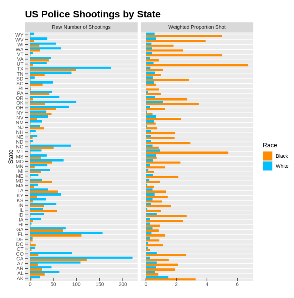
Evidently, despite the fact that the actual number of white victims is significantly larger than that of Black victims nation-wide, the number of individuals shot per million in each state is actually far greater with regards to the Black population. This finding confirms the prevalence of racial disparity in police violence across the US, suggesting that Black Americans are in fact at greater risk of being victimized by police compared to whites.
IV. Analysis
To explore the racial discrepancies in number of individuals shot by police relative to state populations, as depicted in the rightmost bar graph of the figure above, we shift our focus to the following two measures:
-
Difference: Difference between the number of Black and white shootings per million in the racial population for state \(j\). \[d_j = x_{bj}-x_{wj}\]
-
Ratio: Ratio of weighted Black to white shootings in state \(j\), i.e., the weighted number of Black victims per white victim. \[r_j = x_{bj}/x_{wj}\]
These metrics provide a way to analyze racial disparities in police shootings by comparing observed rates relative to one another and to the degree of state-wide police violence documented. Specifically, while differences shed light on these discrepancies as it pertains to the sheer number of victims, ratios provide a more stark comparison of shooting rates, ignoring the magnitude of police brutality present in each state. For each of the two measures we construct a bar graph, violin plot and US map, as depicted below, to visualize and better gauge these racial disparities as they relate to geographical location and political climate at the state level.
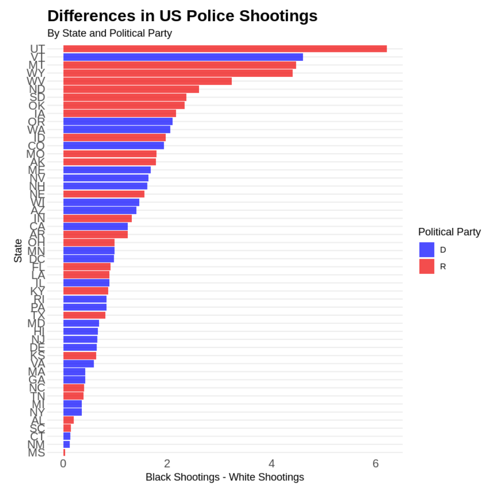
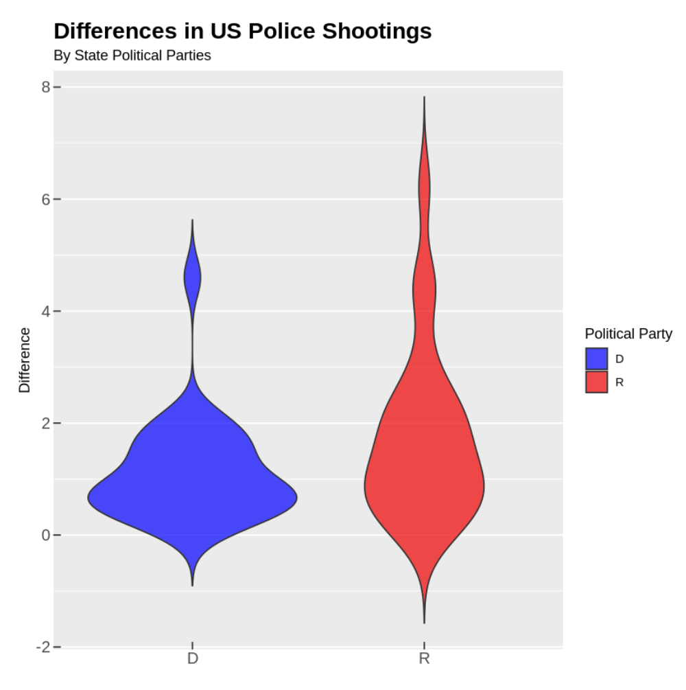
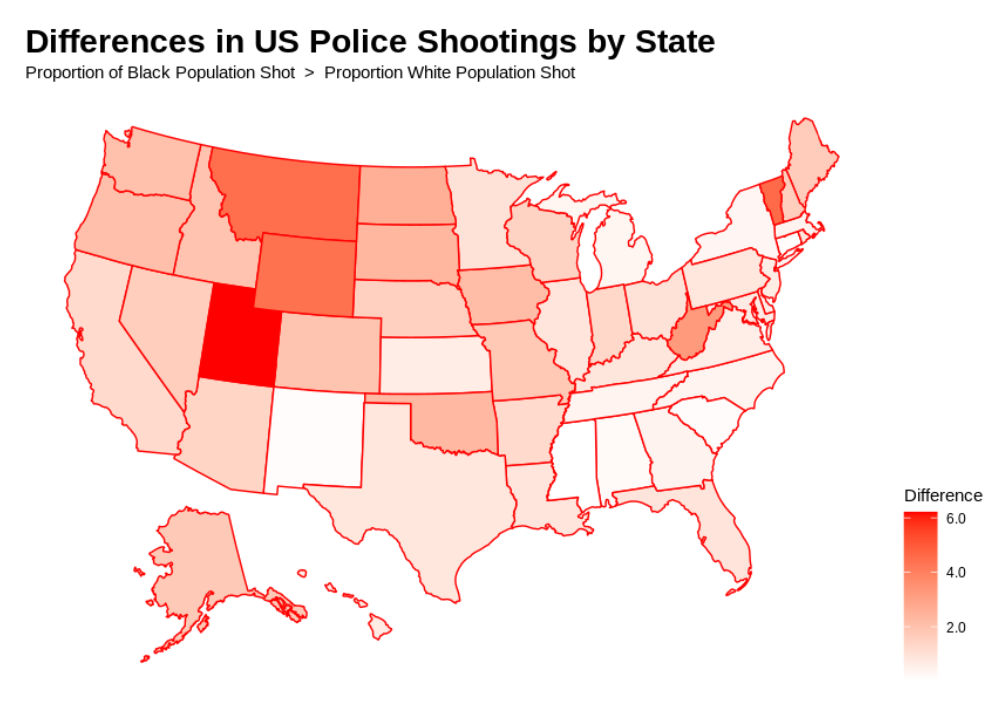
From these graphs, it can be noticed that 8 out of the 10 most significant differences in police shootings over the last five years belonged to red states, the largest of which was documented in UT—the second most Republican state in the US, according to the World Population Review. Moreover, the bar graph shows that the second largest discrepancy corresponds to Vermont, which despite being a blue state, is among the most racist states in the country, as found by the World Population Review. Trailing behind these are Montana, Wyoming, West Virginia, North Dakota, South Dakota, Oklahoma, and Iowa—all red states of which 5 are among the 10 most Republican in the country, according to the same article. Despite not offering definitive proof of a relationship between political climate and racial disparity in police violence, this information substantiates our findings, suggesting a potential influence of political climate on both the frequency of shootings and the racial gap in police brutality.
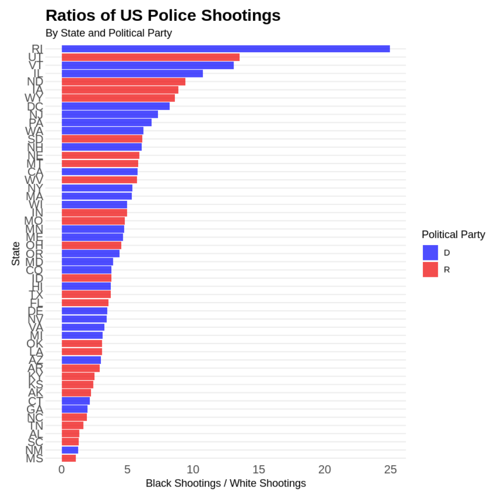
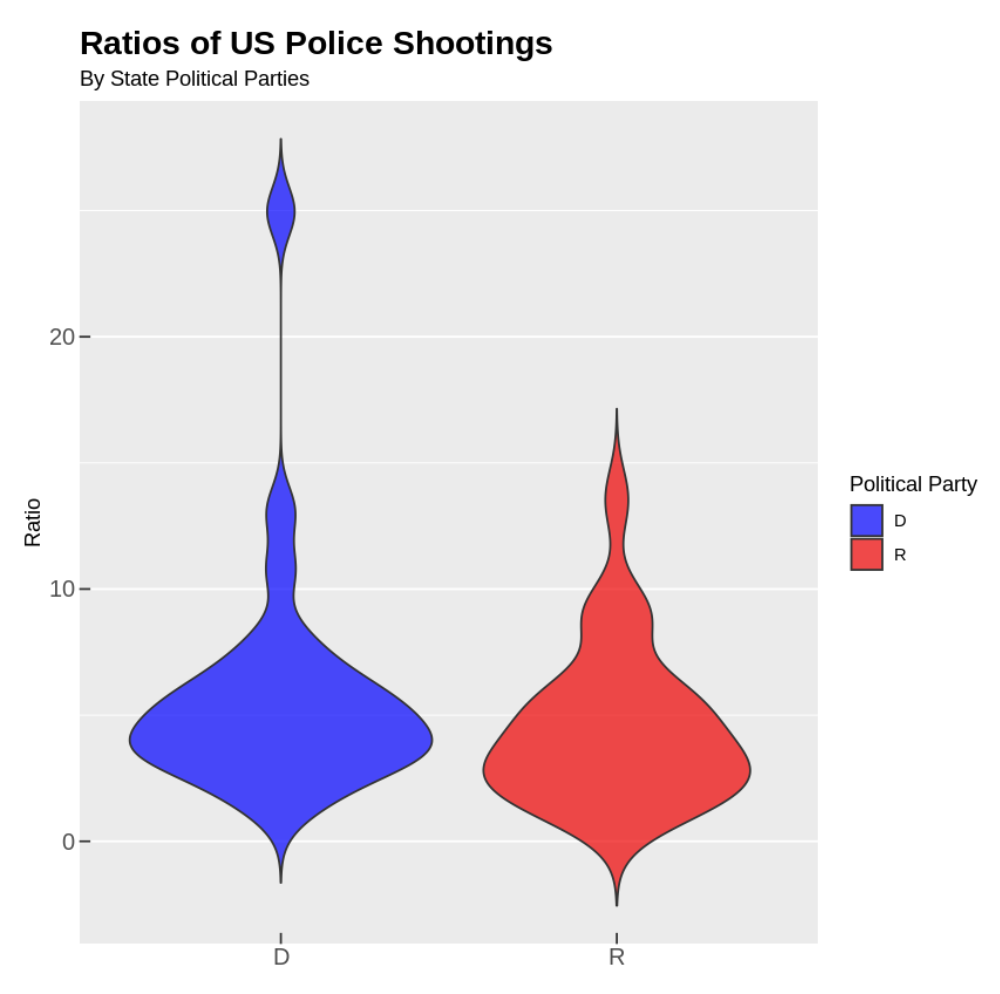
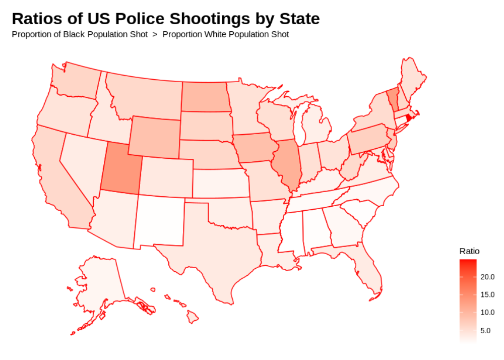
These visualizations reflect the weighted ratios of Black to white shootings, illustrating the relative difference in documented police violence across blue and red states. Specifically, it can be seen from the first two graphs that discrepancies are more evenly distributed between political parties, with the exception of RI—a potential outlier due to sample size, which displayed the largest ratio of Black to white shootings. However, it is evident that, with the exception of RI, the states with the two highest relative disparities in police shootings are UT and VT—states that demonstrated equally significant racial differences in number of shootings and have been found to possess strong conservative and racist ties.
As mentioned, differences \(d_j\) allow us to visualize statewide disparities taking into account the degree of police violence evidenced, meanwhile ratios \(r_j\) provide a sense for how large this gap is irrespective of the number of documented shootings. For example, although UT displays a much more considerable discrepancy in police shootings compared to RI, RI exhibits a greater relative difference in violence between races. However, we note that given large contrasts in area, population and number of observed instances between states, it is possible for smaller samples to have produced misleeding estimates. Thus, it is important to consider the potential influence of sampling on our results, take note of vast inconsitancies between metrics, and utilize both measures in tandem to form inferences about the nature of racial disparity in police violence across the country.
V. Conclusion
Based on our analysis of police shooting data from the past five years, specifically with regards to Black and white US populations, we can be certain of a clear racial gap in national police violence. Moreover, our findings suggest that race is a significant risk factor for police brutality, which varies between states of oppossing political climates. Specifically, not only does the number of Black Americans shot by police relative to the population exceed that of whites in every state, but the extent of the discrepancy is likely tied to a state’s dominant political party and its views on race. Moreover, while ratios show that law enforcement across blue and red states display similar levels of discrimination against Black individuals, more conservative political climates appear to exacerbate these differences when considering the amount of police violence present in a given area. Thus, we suspect that in addition to Black Americans facing greater risks of being harmed by police, individuals living in areas heavily dominated by conservative and/or racist ideologies may have additional risks associated with higher frequencies of documented police brutality. The information gathered here paints a rather grim picture of our nation’s criminal justice system. Not only does it shed light on the racism embedded within our institutions, but it demonstrates how conservative ideologies which parallel inegalitarian beliefs may aggrandize and perpetuate these injustices. For this reason, radical action and intervention is needed, in addition to public awareness, to combat racial injustice and thus, preserve the country’s commitment to equality and democracy. This work, more than quantifying the level of racism present in the US police system, speaks to the power of data to both mask and expose the issues that plague our society. Analyses like this one lend weight to the vital importance of ethical data collection, processing, and representation, which are key to raising awareness and catalyzing positive societal and institutional changes.
Code Appendix
## Libraries
library(tidyverse)
library(usmap)
## Preprocessing Data

# police shootings data
shootings <- read.csv('~/shootings.csv') %>%
   select(-c(id, armed))

# state population/demographic data
demo_data <- read.delim('~/Bridged-Race Population Estimates 1990-2020.txt') %>%
   na.omit() %>%
   select(State, Race, Population)
demo_data$Race <- sub("^$", "Total", demo_data$Race)
demo_data_rm <- filter(Race != "Total")
demo_data_tot <- demo_data %>%
   pivot_wider(names_from=Race, values_from=Population) %>%
   select(c("State", "Total"))
demo <- demo_data_rm %>%
   full_join(demo_data_tot, by="State") %>%
   rename(state=State, race=Race, sub_pop=Population, total_pop=Total)

# converting state names to abbreviations for merging with shootings data
demo$state <- gsub("West VA", "West Virginia", demo$state)
demo$state <- state.abb[match(demo$state, state.name)]
for (i in 1:length(demo$state)){ # DC is converted to 'NA' by default
  if (is.na(demo$state[i])){
    demo$state[i] <- "DC"
  }
}

# renaming race values
demo$race <- gsub("Black or African American", "Black", demo$race)

# merging data
us_shootings <- shootings %>%
   full_join(demo, by=c("state", "race"))
bw_shootings %>% us_shootings %>%
   filter(race == "Black" | race == "White") # populations of interest
# how many Black vs. white shootings?
table(bw_shootings$race)
nrow(bw_shootings) # total number of Black and White shootings (~35% Black, ~65% white)
nrow(us_shootings) # total number of shootings (~27% Black, ~50% white)
## Weighting

# df of number of shootings in each state by race
grouped_bw_shootings <- bw_shootings %>%
   group_by(state, race) %>%
   count() %>%
   left_join(demo, by=c("state", "race"))

# adding population and weighted observation metric columns
BLM <- grouped_bw_shootings %>%
    mutate(sub_pop_mill = sub_pop/1000000, weighted_prop_shot = n/sub_pop_mill)
# Figure 1

# comparing raw and weighted number of shootings
rw_shootings <- BLM %>%
   select(state, race, n, weighted_prop_shot) %>%
   pivot_longer(!(state|race), names_to = "type_prop", values_to = "count")

# new facet label names for type_prop variable
type_prop.labs <- c("Raw Number of Shootings", "Weighted Proportion Shot")
names(type_prop.labs) <- c("n", "weighted_prop_shot")

ggplot(data=rw_shootings, aes(x=state, y=count, fill=race)) +
   geom_bar(stat="identity", position=position_dodge(), alpha=1) +
   facet_wrap(~type_prop, scales="free_x", labeller=labeller(type_prop=type_prop.labs)) +
   coord_flip() +
   scale_fill_manual(values=c("darkorange", "deepskyblue1"), name="Race") +
   labs(x="State", title="US Police Shootings by State") +
   theme(panel.grid.major.x=element_blank(),
         panel.grid.minor.x=element_blank(),
         axis.ticks.length=unit(-0.2, "cm"),
         axis.title.y=element_blank(),
         plot.title=element_text(face="bold", size=17))
## Analysis (Racial Disparities)

# including state political affiliations
state <- unique(BLM$state)

# red states
R <- c("AK", "AL", "AR", "FL", "IA",
       "ID", "IN", "KS", "KY", "LA",
       "MO", "MS", "MT", "NC", "ND",
       "NE", "OH", "OK", "SC", "SD",
       "TN", "TX", "UT", "WV", "WY")

pol_party <- c()
for (i in 1:length(states)){
   if (states[i] %in% R){
      pol_party[i] <- "R"
      } else{
           pol_party[i] <- "D"
        }
   }

# 1. DIFFERENCE: xb-xw
diff <- c()
for (i in 1:(nrow(BLM)-1)){
   if (BLM$state[i] == BLM$state[i+1]){
      if (BLM$weighted_prop_shot[i] > BLM$weighted_prop_shot[i+1]){
         diff <- c(diff, BLM$weighted_prop_shot[i]-BLM$weighted_prop_shot[i+1])
         }
      }
   }
BLM_diff <- data.frame(state, pol_party, diff)
BLM_diff <- arrange(BLM_diff, desc(diff))

# 2. RATIO: xb/xw
ratio <- c()
for (i in 1:(nrow(BLM)-1)){
   if (BLM$state[i] == BLM$state[i+1]){
      if (BLM$weighted_prop_shot[i] > BLM$weighted_prop_shot[i+1]){
         ratio <- c(ratio, BLM$weighted_prop_shot[i]/BLM$weighted_prop_shot[i+1])
         }
      }
   }
BLM_ratio <- data.frame(state, pol_party, ratio)
BLM_ratio <- arrange(BLM_ratio, desc(ratio))
## Visualizing Racial Disparities - DIFFERENCES

# bar graph (Figure 2)
ggplot(BLM_diff, aes(x=reorder(state, diff), y=diff, fill=pol_party)) +
   geom_bar(stat="identity", alpha=0.7) +
   scale_fill_manual(values=c("blue", "red2"), name="Political Party") +
   labs(x="State", y="Black Shootings - White Shootings",
        title="Differences in US Police Shootings",
        subtitle="By State and Political Party") +
   coord_flip() +
   theme_minimal() +
   theme(panel.grid.major.x=element_blank(),
         axis.text=element_text(size=12),
         axis.ticks.length=unit(-0.2, "cm"),
         plot.title=element_text(face="bold", size=17))

# violin plot (Figure 3)
ggplot(BLM_diff, aes(x=pol_party, y=diff, fill=pol_party)) +
   geom_violin(trim=FALSE, alpha=0.7) +
   scale_fill_manual(values=c("blue", "red2"), name="Political Party") +
   labs(y="Difference",
        title="Differences in US Police Shootings",
        subtitle="By Political Party") +
   theme(panel.grid.major.x=element_blank(),
         axis.text=element_text(size=12),
         axis.ticks.length=unit(-0.2, "cm"),
         axis.title.x=element_blank(),
         plot.title=element_text(face="bold", size=17))

# US map (Figure 4)
plot_usmap(data=BLM_diff, values="diff", color="red") +
   scale_fill_continuous(low="white", high="red", name="Difference", label=scales::comma) +
   labs(title="Differences in US Police Shootings by State",
        subtitle="Proportion of Black Population Shot > Proportion of White Population Shot") +
   theme(legend.position="right",
         panel.grid.major.x=element_blank(),
         axis.ticks.length=unit(-0.2, "cm"),
         plot.title=element_text(face="bold", size=17))
## Visualizing Racial Disparities - RATIOS

# bar graph (Figure 5)
ggplot(BLM_ratio, aes(x=reorder(state, ratio), y=ratio, fill=pol_party)) +
   geom_bar(stat="identity", alpha=0.7) +
   scale_fill_manual(values=c("blue", "red2"), name="Political Party") +
   labs(x="State", y="Black Shootings / White Shootings",
        title="Ratios of US Police Shootings",
        subtitle="By State and Political Party") +
   coord_flip() +
   theme_minimal() +
   theme(panel.grid.major.x=element_blank(),
         axis.text=element_text(size=12),
         axis.ticks.length=unit(-0.2, "cm"),
         plot.title=element_text(face="bold", size=17))

# violin plot (Figure 6)
ggplot(BLM_ratio, aes(x=pol_party, y=ratio, fill=pol_party)) +
   geom_violin(trim=FALSE, alpha=0.7) +
   scale_fill_manual(values=c("blue", "red2"), name="Political Party") +
   labs(y="Ratio",
        title="Ratios of US Police Shootings",
        subtitle="By Political Party") +
   theme(panel.grid.major.x=element_blank(),
         axis.text=element_text(size=12),
         axis.ticks.length=unit(-0.2, "cm"),
         axis.title.x=element_blank(),
         plot.title=element_text(face="bold", size=17))

# US map (Figure 7)
plot_usmap(data=BLM_ratio, values="ratio", color="red") +
   scale_fill_continuous(low="white", high="red", name="Ratio", label=scales::comma) +
   labs(title="Ratios of US Police Shootings by State",
        subtitle="Proportion of Black Population Shot > Proportion of White Population Shot") +
   theme(legend.position="right",
         panel.grid.major.x=element_blank(),
         axis.ticks.length=unit(-0.2, "cm"),
         plot.title=element_text(face="bold", size=17))