I. Building, Training and Evaluating a Model
We will be working with a dataset from Folktables, a Python package that provides access to datasets derived from the US Census. The data provided by this library is sourced from the American Community Survey, a demographics survey program that gathers information about individuals’ educational attainment, income, employment, demographic information, etc. First, we download and process a dataset from California 2018.
Specifically, we focus the ACSPublicCoverage binary classification task, as defined by Folktables, which seeks to predict whether individuals have public coverage based on a given a set of features (i.e., age, sex, race, and a range of disabilities). Given that one of the features used in prediction is the race sensitive attribute, which should have no correlation with the outcome, our goal is to utilize different techniques to make our model more fair in its prediction.
A. Data & Preprocessing
We first begin by observing the data.
from folktables import ACSDataSource, ACSPublicCoverage

# import data source form ACS
data_source = ACSDataSource(survey_year='2018', horizon='1-Year', survey='person')
acs_data = data_source.get_data(states=["CA"], download=True)
prediction_task = ACSPublicCoverage

# gather columns defined in the ACSPublicCoverage prediction task
features, label, group = prediction_task.df_to_numpy(acs_data)

# aggregate features and target variable into the same dataframe
acs_public_coverage_data = acs_data[prediction_task.features + [prediction_task.target]]

## data summary
print(acs_public_coverage_data.head())
print("features used for predictions: "   + str(prediction_task.features))
print("group membership variable: "       + str(prediction_task.group))
print("the target variable of interest: " + str(prediction_task.target))
    AGEP  SCHL  MAR  SEX  DIS  ESP  CIT  MIG  MIL  ANC  NATIVITY  DEAR  DEYE  \
0    30  14.0    1    1    2  NaN    1  3.0  4.0    1         1     2     2
1    18  14.0    5    2    2  NaN    1  1.0  4.0    1         1     2     2
2    69  17.0    1    1    1  NaN    1  1.0  2.0    2         1     2     2
3    25   1.0    5    1    1  NaN    1  1.0  4.0    1         1     1     2
4    31  18.0    5    2    2  NaN    1  1.0  4.0    1         1     2     2

   DREM    PINCP  ESR  ST  FER  RAC1P  PUBCOV
0   2.0  48500.0  6.0   6  NaN      8       1
1   2.0      0.0  6.0   6  2.0      1       2
2   2.0  13100.0  6.0   6  NaN      9       1
3   1.0      0.0  6.0   6  NaN      1       1
4   2.0      0.0  6.0   6  2.0      1       1

features used for predictions: ['AGEP', 'SCHL', 'MAR', 'SEX', 'DIS', 'ESP', 'CIT', 'MIG', 'MIL', 'ANC', 'NATIVITY', 'DEAR', 'DEYE', 'DREM', 'PINCP', 'ESR', 'ST', 'FER', 'RAC1P']
group membership variable: RAC1P
the target variable of interest: PUBCOV
import matplotlib.pyplot as plt
## data visualization
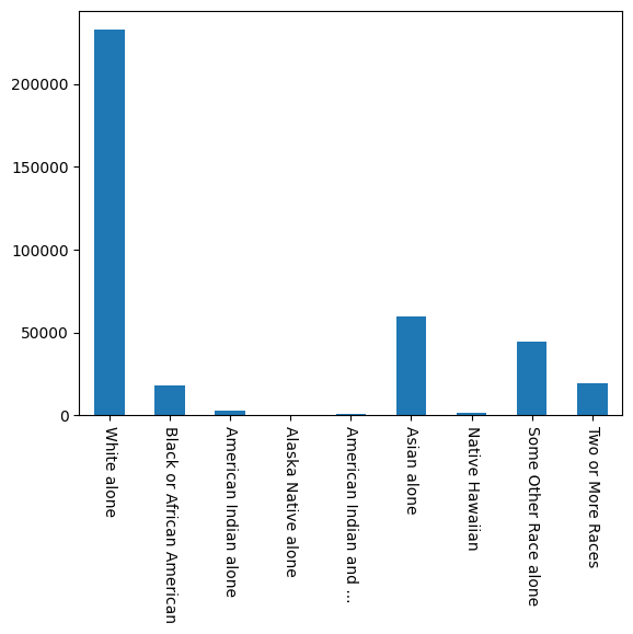
race_coding = [
'White alone', # white alone
'Black or African American', # black or african american alone
'American Indian alone', # american indian alone
'Alaska Native alone', # alaska native alone
'American Indian and ...', # american indian and alaska native tribes specified;
# or american indian and alaska native not specified, and no other races
'Asian alone', # asian alone
'Native Hawaiian', # native hawaiian and other pacific islander alone
'Some Other Race alone', # some other race alone
'Two or More Races'] # two or more races
# bar graph by group membership
(acs_public_coverage_data
.groupby([prediction_task.group])
.size()
.set_axis(race_coding)
.plot(kind='bar', rot=-90))
health_coverage_coding = ['With public health coverage', 'Without public health coverage']

# bar graph by target of interest
(acs_public_coverage_data
 .groupby([prediction_task.target])
 .size()
 .set_axis(health_coverage_coding)
 .plot(kind='bar', rot=0))
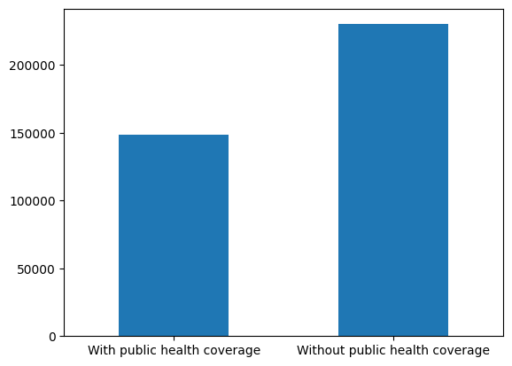
Both bar graphs reflect that neither the race class nor the target label are balanced (i.e., evently distributed), displaying significant differences within them.
B. Training
We now define our training function with logistic regression, using the make_pipeline and StandardScaler() functions to initialize the model.
def train(X_train, y_train):
  """
  Defines and trains a logistic regression model on the training data.

  Args:
    X_train (np.ndarray): Training inputs.
    y_train (np.ndarray): Training labels.

  Returns:
    sklearn.pipeline.Pipeline: trained model
  """
  # TODO: train model

  LR_pipeline = make_pipeline(StandardScaler(), LogisticRegression()).fit(X_train, y_train)
  return LR_pipeline
C. Evaluation
Implementing the three fairness measurements discussed in Fairness and Machine Learning: Limitations and Opportunities and defined below—independence, separation and sufficiency, we can evalute how fair our model is in predicting status of public health coverage.
Let \(Y\) be the binary target variable, \(\hat{Y}\) be the model’s predicted outcome and \(A\) be some sensitive attiribute.
- Random variables \((A, \hat{Y})\) satisty independence, i.e., \(A \perp \hat{Y}\), if
\[\frac{P\{ \hat{Y} = 1\ | A = a\}}{P\{ \hat{Y} = 1\ | A = b\}} = 1.\]
- Random variables \((A, Y, \hat{Y})\) satisty separation, i.e., \(A \perp \hat{Y} \mid Y\), if for groups in \(A\), say \(a\) and \(a’\),
\[\frac{P\{ \hat {Y} | Y = 1, A = a\}} {P \{\hat{Y} | Y = 1, A = a'\}} = 1;\]
\[\frac{P\{ \hat {Y} | Y = 0, A = a\}} {P \{\hat{Y} | Y = 0, A = a'\}} = 1.\]
- Random variables \((A, Y, \hat{Y})\) satisty sufficiency, i.e., \(A \perp Y \mid \hat{Y}\), iff for all values \(\hat{y}\) of \(\hat{Y}\) and groups in \(A\), say \(a\) and \(a’\),
\[\frac{P\{Y = 1 | \hat{Y} = \hat{y}, A = a\}}{P\{Y = 1 | \hat{Y} = \hat{y}, A = a'\}} = 1.\]
(NOTE: Separation is the same as equalizing true positive and false positive rates accross groups.)
from operator import index

# independence
def independence(y_hat, group):
  """
  Computes an independence metric between two groups.

  Args:
    y_hat (np.ndarray): Classifier predictions.
    group (np.ndarray): Array of indices corresponding to group membership.
      For our purposes, we focus on comparing groups 1 and 2. These correspond
      to the 'White alone' and 'Black or African American' groups.

  Returns:
    float: independence measure
  """
  # TODO: compute measure

  idx1 = np.where(group == 1)[0]
  idx2 = np.where(group == 2)[0]

  P1 = sum(y_hat[(idx1),])/len(y_hat[(idx1),])
  P2 = sum(y_hat[(idx2),])/len(y_hat[(idx2),])

  indep = P2/P1
  return indep

# separation
def separation(y_hat, y_true, group):
  """
  Computes a separation metric between two specific groups.

  Args:
    y_hat  (np.ndarray): Classifier predictions.
    y_true (np.ndarray): Data labels.
    group  (np.ndarray): Array of indices corresponding to group membership.
      For our purposes, we focus on comparing groups 1 and 2. These correspond
      to the 'White alone' and 'Black or African American' groups.

  Returns:
    float: separation true positive
    float: separation false positive
  """
  # TODO: compute measure

  idx1_1 = np.intersect1d(np.where(y_true == 1)[0], np.where(group == 1)[0])
  idx1_2 = np.intersect1d(np.where(y_true == 1)[0], np.where(group == 2)[0])
  idx0_1 = np.intersect1d(np.where(y_true == 0)[0], np.where(group == 1)[0])
  idx0_2 = np.intersect1d(np.where(y_true == 0)[0], np.where(group == 2)[0])

  P1_1 = sum(y_hat[(idx1_1),])/len(y_hat[(idx1_1),])
  P1_2 = sum(y_hat[(idx1_2),])/len(y_hat[(idx1_2),])

  P0_1 = sum(y_hat[(idx0_1),])/len(y_hat[(idx0_1),])
  P0_2 = sum(y_hat[(idx0_2),])/len(y_hat[(idx0_2),])

  TP = P1_2/P1_1
  FP = P0_2/P0_1
  return TP, FP

# sufficiency
def sufficiency(y_hat, y_true, group):
  """
  Computes a sufficiency metric between two specific groups.

  Args:
    y_hat  (np.ndarray): Classifier predictions.
    y_true (np.ndarray): Data labels.
    group  (np.ndarray): Array of indices corresponding to group membership.
      For our purposes, we focus on comparing groups 1 and 2. These correspond
      to the 'White alone' and 'Black or African American' groups.

  Returns:
    float: sufficiency metric
  """
  # TODO: compute metric

  idx1_1 = np.intersect1d(np.where(y_hat == 1)[0], np.where(group == 1)[0])
  idx1_2 = np.intersect1d(np.where(y_hat == 1)[0], np.where(group == 2)[0])

  P1_1 = sum(y_true[(idx1_1),])/len(y_true[(idx1_1),])
  P1_2 = sum(y_true[(idx1_2),])/len(y_true[(idx1_2),])

  suff = P1_2/P1_1
  return suff

# evaluation function
def eval(yhat, y_test, group_test, model_title):
  print("Results from the " + model_title + " model: ")
  print("the indepence of prediction and group is ", independence(yhat, group_test))
  true_s, false_s = separation(yhat, y_test, group_test)
  print("the true positive separation is ", true_s)
  print("the false positive separation is ", false_s)
  print("the sufficiency of the prediction and the group is", sufficiency(yhat, y_test, group_test))

y_hat_example = np.asarray([True, True, False, False, True, False, False, False, True, True])
y_test_example = np.asarray([True, True, True,  False, False, False, False, True, False, True])
group_test_example = np.asarray([1, 1, 1, 1, 1, 2, 2, 2, 2, 2])

eval(y_hat_example, y_test_example, group_test_example, "unit-test")
Results from the unit-test model:
the indepence of prediction and group is  0.6666666666666667
the true positive separation is  0.75
the false positive separation is  0.6666666666666666
the sufficiency of the prediction and the group is 0.75
D. The Full Workflow
Finally, we connect the whole pipeline with training and see how fair our model is. We will:
- Do an 80-20
train_test_split on the dataset with random_state = 0.
- Train our linear regression model.
- Use the trained model to make predictions on the test dataset.
- Evaluate the model with fairness measurements.
# split the data into training and testing sets
X_train, X_test, y_train, y_test, group_train, group_test = train_test_split(
    features, label, group, test_size=0.2, random_state=0)
model = train(X_train, y_train)
yhat = model.predict(X_test)

eval(yhat, y_test, group_test, "baseline")
Results from the baseline model:
the indepence of prediction and group is  1.6135056165484982
the true positive separation is  1.3052337292915481
the false positive separation is  1.2975609756097561
the sufficiency of the prediction and the group is 1.196133899104196
II. Resampling
We now retrain our model using inputs that have a different ratio of elements in demographic groups to observe how the fairness measures change. That is, by modifying the frequency at which different groups appear in the training set. To achieve this, we implement the uniform sampling method described in Algorithm 4 of Data Preprocessing Techniques for Classification Without Discrimination, wherein the chance of sampling any given point within a group is uniform. As described, “all the data objects of the same group have the same chance of being duplicated or skipped”.
Section 5.3 details the partitioning of the dataset into various groups of interest. Specifically, our goal is to rebalance these groups, while maintaining the total number of training data points the same, such that some observations are skipped and others duplicated. We achieve this by implementing a weighting approach to calculate the necessary sample weights for each group according to the formulas described in the paper.
## Weighting Approach
def compute_sample_weight(y, group):
  """
  Computes sample weights according to the algorithm described in the paper.

  Args:
    y     (np.ndarray): Training labels.
    group (np.ndarray): Array of indices corresponding to group membership.

  Returns:
    list: sample weight
    dict: weight dict
  """
  assert(len(y) == len(group))

  # TODO: calculate sample weight

  name_keys = ["N1", "N2", "P1", "P2"]
  weight_values = []

  for i in np.unique(y):
    for j in np.unique(group):
      numer = len(np.where(y == i)[0])*len(np.where(group == j)[0])
      denom = len(y)*len(np.intersect1d(np.where(y == i)[0], np.where(group == j)[0]))
      weight = numer/denom
      weight_values.append(weight)

  weight_dict = dict(map(lambda k,v : (k,v), name_keys, weight_values))

  sample_weight = []

  for p in range(len(y)):
    if y[p] == 0:
      if group[p] == 1:
        sample_weight.append(weight_dict["N1"])
      else:
        sample_weight.append(weight_dict["N2"])
    elif y[p] == 1:
      if group[p] == 1:
        sample_weight.append(weight_dict["P1"])
      else:
        sample_weight.append(weight_dict["P2"])

  return sample_weight, weight_dict

# NOTE: We later use `sample_weight` in cost-sensitive learning
#       and `weight_dict` in uniform sampling

sample_weight, weight_dict = compute_sample_weight(y_train, group_train)
print(weight_dict)
{'N1': 0.980464144062951, 'N2': 1.2972056964427827, 'P1': 1.1403499657377425, 'P2': 0.981331954005014}
## Uniform Sampling
def uniform_sampling(X, y, group, weight_dict):
  """
  Perform uniform sampling given a `weight_dict`

  Args:
    X     (np.ndarray): Training data.
    y     (np.ndarray): Training labels.
    group (np.ndarray): Array of indices corresponding to group membership.
    weight_dict (dict): Dict containing weights for different groups.

  Returns:
    np.ndarray: Sampled training data
    np.ndarray: Corresponding sampled training labels
    np.ndarray: Corresponding sampled array of group membership
  """
  # TODO: perform uniform sampling

  idx_N1 = np.intersect1d(np.where(y == 0)[0], np.where(group == 1)[0])
  idx_N2 = np.intersect1d(np.where(y == 0)[0], np.where(group == 2)[0])
  idx_P1 = np.intersect1d(np.where(y == 1)[0], np.where(group == 1)[0])
  idx_P2 = np.intersect1d(np.where(y == 1)[0], np.where(group == 2)[0])

  samp_size_N1 = round(weight_dict["N1"]*len(idx_N1))
  samp_size_N2 = round(weight_dict["N2"]*len(idx_N2))
  samp_size_P1 = round(weight_dict["P1"]*len(idx_P1))
  samp_size_P2 = round(weight_dict["P2"]*len(idx_P2))

  samp_idx_N1 = [np.random.choice(idx_N1) for i in range(samp_size_N1)]
  samp_idx_N2 = [np.random.choice(idx_N2) for i in range(samp_size_N2)]
  samp_idx_P1 = [np.random.choice(idx_P1) for i in range(samp_size_P1)]
  samp_idx_P2 = [np.random.choice(idx_P2) for i in range(samp_size_P2)]

  samp_indices = samp_idx_N1 + samp_idx_N2 + samp_idx_P1 + samp_idx_P2

  X_sampled = X[samp_indices]
  y_sampled = y[samp_indices]
  group_sampled = group[samp_indices]

  return X_sampled, y_sampled, group_sampled

# sample from training data
X_sampled, y_sampled, group_sampled = uniform_sampling(X_train, y_train, group_train, weight_dict)

model = train(X_sampled, y_sampled)
yhat = model.predict(X_test)
eval(yhat, y_test, group_test, "uniform_sampling")
Results from the uniform_sampling model:
the indepence of prediction and group is  1.5481312022885463
the true positive separation is  1.30027948616628
the false positive separation is  1.1860036832412522
the sufficiency of the prediction and the group is 1.2419123309342532
III. Cost-Sensitive Learning
Lastly, we train our model using a different measure of cost—not accuracy, but cost-sensitive accuracy—to observe what happens to the output. We refer to the LogisticRegression classifier documentation for guidance.
def train_weighted(X_train, y_train):
  """
  Defines and trains a logistic regression model on the training data.
  Applies weighting on training the model.

  Args:
    X_train (np.ndarray): Training inputs.
    y_train (np.ndarray): Training labels.

  Returns:
    sklearn.pipeline.Pipeline: trained model
  """
  # TODO: train model

  sample_weights = np.array(compute_sample_weight(y_train, group_train)[0])

  LR_pipeline = make_pipeline(StandardScaler(), LogisticRegression())
  model_train = LR_pipeline.fit(X_train, y_train,
                                logisticregression__sample_weight = sample_weights)

  return model_train
weighted_model = train_weighted(X_train, y_train)
yhat = weighted_model.predict(X_test)
eval(yhat, y_test, group_test, "weighted")
Results from the weighted model:
the indepence of prediction and group is  1.5036432659126076
the true positive separation is  1.2457235915065032
the false positive separation is  1.1630769230769231
the sufficiency of the prediction and the group is 1.2250078385288548